Tema 2: Análisis multivariado de series temporales⁽³⁾

Curso: Tópicos Avanzados de Series Temporales

Shu Wei Chou Chen

shuwei.chou@ucr.ac.cr

Escuela de Estadística, Universidad de Costa Rica

VARX(p)

Contenido

VARX(p)
Ejemplo simulado
Pronóstico
El análisis del impulso-respuesta
Ejemplo

VARX(p)

Vamos a enfocarnos en el modelo VAR(p) con posibilidad de incluir covariables (variables exógenas):

\[X_{t}=CD_t+\phi_1 X_{t-1}+...+\phi_pX_{t-p}+a_{t}\] donde \(\phi_0\) es un vector de dimensión \(k\), \(\phi_i\) matrices \(k \times k\) para \(i=1,...,p\), \(\phi_p \neq 0\) y \(a_t\) es una secuencia de i.i.d. vectores aleatorios con media 0 y matriz de covariancias \(\Sigma_a\), que es definida positiva, \(C\) es la matriz de coeficientes de dimiensión \((k \times M)\) y \(D_t\) es el vector columna de variables exógenas \((M \times 1)\).

Su representación con el operador autorregresivo es \[\phi(B) X_{t}=CD_t+a_{t}\] donde \(\phi(B)=I_k- \phi_1 B-...- \phi_p B^p\) es el operador autorregresivo.
Si las soluciones de \(|\phi(B)|\), están fuera del círculo unitario, entonces VARX(p) es estacionario.

VARX(1)

VARX(1) con 3 series tepmorales y variables exógenas: intercepto y tendencia.

\[X_{t}=C D_t+\phi X_{t-1}+a_{t},\]

\[\text{donde}~~ C=\begin{bmatrix}\alpha_{1} & \beta_{1} \\ \alpha_{2} & \beta_{2} \\ \alpha_{3} & \beta_{3} \end{bmatrix} ~~\text{y}~~ D_t= \begin{bmatrix}1 \\ t \end{bmatrix}\]

Es decir,

\[X_{1,t}=\alpha_1 + \beta_1 t+\phi_{11}X_{1,t-1}+\phi_{12}X_{2,t-1}+\phi_{13}X_{3,t-1}+a_{1,t}\]

\[X_{2,t}=\alpha_2+ \beta_2 t+\phi_{21}X_{1,t-1}+\phi_{22}X_{2,t-1}+\phi_{23}X_{3,t-1}+a_{2,t}\]

\[X_{3,t}=\alpha_3+ \beta_3 t+\phi_{31}X_{1,t-1}+\phi_{32}X_{2,t-1}+\phi_{33}X_{3,t-1}+a_{3,t}\] # Causalidad de Granger

Causalidad de Granger de un VAR(1)

Considere el modelo VAR(1):

\[X_{t}=\phi_0+\phi_1 X_{t-1} + a_{t}\] - Expresando explícitamente la ecuación,

\[\begin{bmatrix}X_{1,t}\\ X_{2,t} \end{bmatrix} =\begin{bmatrix}\phi_{10}\\ \phi_{20} \end{bmatrix} + \begin{bmatrix}\phi_{1,11} & \phi_{1,12} \\ \phi_{1,21} & \phi_{1,22} \end{bmatrix} \begin{bmatrix}X_{1,t-1}\\ X_{2,t-1} \end{bmatrix} +\begin{bmatrix}a_{1,t}\\ a_{2,t} \end{bmatrix}\]

O bien,

\[X_{1,t}=\phi_{10}+\phi_{1,11}X_{t-1,1}+\phi_{1,12}X_{t-1,2}+a_{1,t}\]

\[X_{2,t}=\phi_{20}+\phi_{1,21}X_{t-1,1}+\phi_{1,22}X_{t-1,2}+a_{2,t}\]

Habíamos discutido que \(X_{1,t}\) causa a \(X_{2,t}\) en el sentido de Granger si \(\phi_{1,21} \neq 0\).

Causalidad de Granger de un VARX(p)

Recordemos que el modelo VARX(p) se puede representar por:

\[X_{t}=CD_t+ \sum_{i=1}^p \phi_i X_{t-i}+a_{t}\]

Podemos representar este modelo por bloques. Considere dos subvectores de \(X_t\), i.e. \(X_t=(\dot{X}_{1,t},\dot{X}_{2,t})\) donde \(\dot{X}_{1,t}\) de dimensión \(k_1\) y \(\dot{X}_{2,t}\) de dimensión \(k_2\) y \(k=k_1+k_2\).

\[\begin{bmatrix}\dot{X}_{1,t}\\ \dot{X}_{2,t} \end{bmatrix} = CD_t + \sum_{i=1}^p \begin{bmatrix}\Phi_{i,11} & \Phi_{i,12} \\ \Phi_{i,21} & \Phi_{i,22} \end{bmatrix} \begin{bmatrix}\dot{X}_{1,t-i}\\ \dot{X}_{2,t-i} \end{bmatrix} +\begin{bmatrix}\dot{a}_{1,t}\\ \dot{a}_{2,t} \end{bmatrix}\]

Note que ahora los elementos de la matriz de coeficientes \(\Phi_{i,12},\Phi_{i,12},\Phi_{i,21},\Phi_{i,22},~i=1,...,p\) son matrices también.

Causalidad de Granger de VAR(1) con \(k=3\)

\[\begin{bmatrix}X_{1,t}\\ X_{2,t}\\ X_{3,t} \end{bmatrix}=\begin{bmatrix}\alpha_{1}\\ \alpha_{2}\\ \alpha_{3} \end{bmatrix}+\begin{bmatrix}\phi_{1,11} & \phi_{1,12} & \phi_{1,13} \\ \phi_{1,21} & \phi_{1,22} & \phi_{1,23}\\ \phi_{1,31} & \phi_{1,32} & \phi_{1,33} \end{bmatrix} \begin{bmatrix}X_{1,t-1}\\ X_{2,t-1}\\ X_{3,t-1} \end{bmatrix}+a_{t}\]

Suponga que nos interesa ver la causalidad de Granger entre \(X_{1,t}\) y \((X_{2,t},X_{3,t})\), i.e. \(X_t=(\dot{X}_{1,t},\dot{X}_{2,t})\) donde \(\dot{X}_{1,t}=X_{1,t}\) y \(\dot{X}_{2,t}=(X_{2,t},X_{3,t})\) con \(k_1=1\) y \(k_2=2\).
En este caso,

\[\Phi_{1,11}=\left[\phi_{1,11}\right],~~\Phi_{1,12}=\left[\phi_{1,12},\phi_{1,13}\right]\] \[\Phi_{1,21}=\begin{bmatrix}\phi_{1,21}\\ \phi_{1,31} \end{bmatrix},~~~\Phi_{1,22}=\begin{bmatrix} \phi_{1,22} & \phi_{1,23}\\ \phi_{1,32} & \phi_{1,33}\end{bmatrix}\]

\[\begin{bmatrix}\dot{X}_{1t}\\ \dot{X}_{2t} \end{bmatrix} = CD_t + \sum_{i=1}^p \begin{bmatrix}\Phi_{i,11} & \Phi_{i,12} \\ \Phi_{i,21} & \Phi_{i,22} \end{bmatrix} \begin{bmatrix}\dot{X}_{1,t-i}\\ \dot{X}_{2,t-i} \end{bmatrix} +\begin{bmatrix}a_{1t}\\ a_{2t} \end{bmatrix}\]

Para contrastar la hipótesis de que el subvector \(\dot{X}_{1t}\) no cause a \(\dot{X}_{2t}\) en el sentido de Granger sería contrastar:

\(H_0:\Phi_{i,21}=0\) para todo \(i=1,...,p\)
\(H_1:\Phi_{i,21} \neq 0\) para algún \(i=1,...,p\).

Considere \(\beta\) el conjunto de todos los parámetros de interés, i.e. todos los elementos de \(\left[\phi_1,...,\phi_p,C\right]\), podemos escribir las restricciones en la siguiente ecuación \[\Gamma \beta=c\] en donde \(\Gamma\) es una matriz \((N \times (k^2p+kM))\).

Para probar la causalidad de Granger, se utiliza el estadístico de Wald para probar la hipótesis. Este estadístico tiene una distribución asintótica de \(F(pk_1k_2,kT-n^*)\) donde \(n^*\) es la cantidad total de parámetros del modelo.
Por otro lado, para probar la causalidad instantánea, se utiliza el estadístico Wald pero con las hipótesis planteadas de la siguiente forma:

\[\begin{align}H_0:&\Gamma \Sigma_a=c \\ H_1:\Gamma \Sigma_a \neq c \end{align}\]

donde \(\Gamma\) es una matriz \((N \times K(K+1)/2)\)

En este caso, el estadístico tiene una distribución asintótica de \(\chi_{N}^2\).

Ejemplo simulado

Contenido

VARX(p)
Ejemplo simulado
Pronóstico
El análisis del impulso-respuesta
Ejemplo

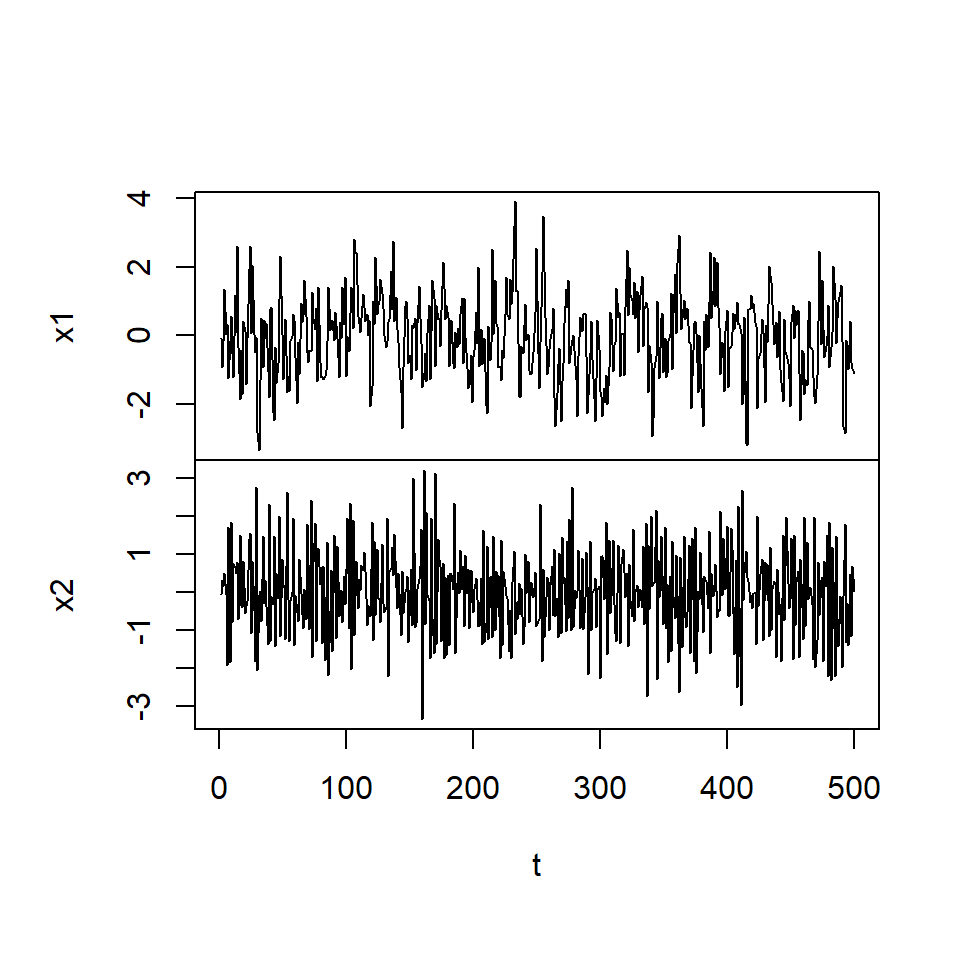
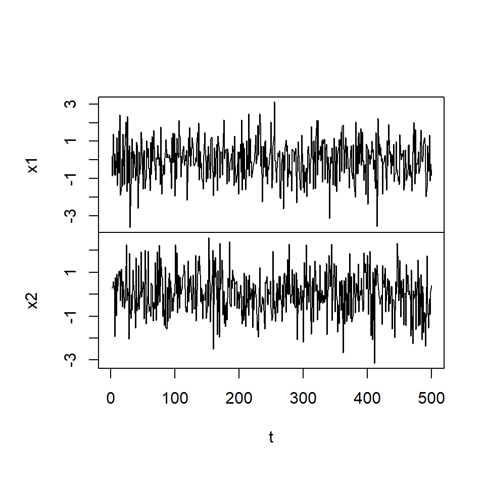
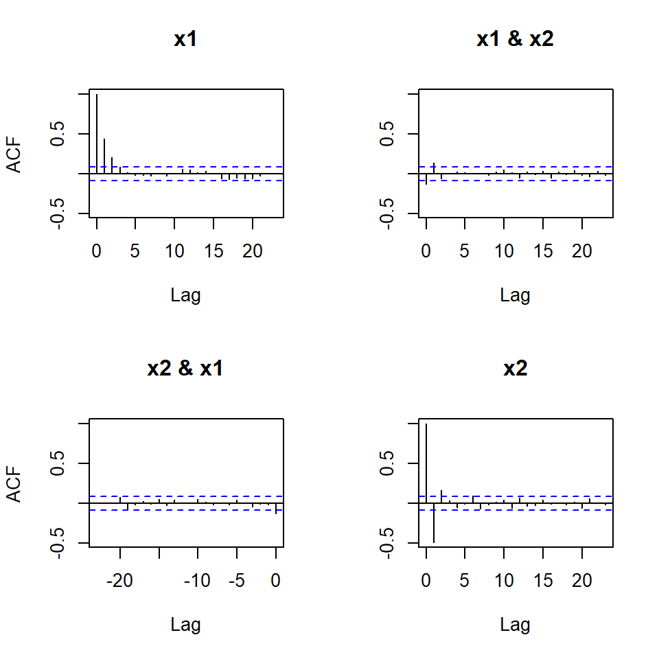
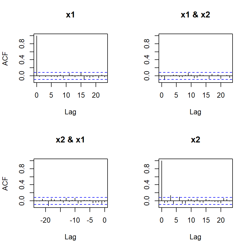
Ejemplo simulado

Considere una realización de \(T=1000\) de un VAR(1):

\[\begin{bmatrix}X_{1t}\\ X_{2t} \end{bmatrix} = \begin{bmatrix} 0.5 & 0.3 \\ 0 & -0.5 \end{bmatrix} \begin{bmatrix}X_{1,t-1}\\ X_{2,t-1} \end{bmatrix} +\begin{bmatrix}a_{1t}\\ a_{2t} \end{bmatrix}\] donde \(a_t \sim N(0,\Sigma_a)\) con \(\Sigma_a=I_2\).

Phi_1 <- matrix(c(0.5, 0.3,
                  0, -0.5), nrow = 2, byrow = TRUE)
Sigma <- diag(2)
simVAR2 <- VARMAsim(nobs = 500, 
                    arlags = c(1), 
                    phi = cbind(Phi_1), 
                    sigma = Sigma)
vardat <- ts(simVAR2$series, names = c("x1", "x2"))
innodat <- ts(simVAR2$noises, names = c("x1", "x2"))

plot.ts(vardat, main = "", xlab = "t")

plot.ts(innodat, main = "", xlab = "t")

stats::acf(vardat)

stats::acf(innodat)

Estimación de modelos

vars::VARselect selecciona el mejor modelo de acuerdo con los diferentes criterios de información.

infocrit <- vars::VARselect(vardat, lag.max = 5,
                      type = "none")
infocrit

$selection
AIC(n)  HQ(n)  SC(n) FPE(n) 
     1      1      1      1 

$criteria
                 1           2           3            4           5
AIC(n) -0.08456655 -0.07853599 -0.06463957 -0.051483956 -0.03925039
HQ(n)  -0.07122862 -0.05186014 -0.02462580  0.001867746  0.02743924
SC(n)  -0.05059032 -0.01058354  0.03728910  0.084420941  0.13063073
FPE(n)  0.91891058  0.92446944  0.93740749  0.949824236  0.96152050

vars::roots verifica que los módulos de los autovalores son menores a 1.

varsimest <- vars::VAR(vardat, p = 1, type = "none",
                 season = NULL, exogen = NULL)
roots <- vars::roots(varsimest)
roots

[1] 0.4907461 0.4606588

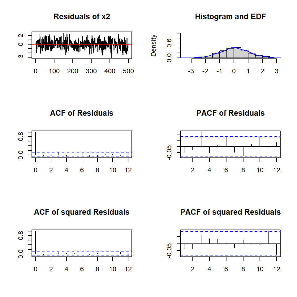
Los diagnósticos

(var.serial <- serial.test(varsimest, lags.pt = 16, type = "PT.asymptotic"))


    Portmanteau Test (asymptotic)

data:  Residuals of VAR object varsimest
Chi-squared = 61.755, df = 60, p-value = 0.4132

(var.arch <- arch.test(varsimest, lags.multi = 5, multivariate.only = TRUE))


    ARCH (multivariate)

data:  Residuals of VAR object varsimest
Chi-squared = 52.264, df = 45, p-value = 0.2126

(var.norm <- normality.test(varsimest, multivariate.only = TRUE))

$JB

    JB-Test (multivariate)

data:  Residuals of VAR object varsimest
Chi-squared = 2.1107, df = 4, p-value = 0.7154


$Skewness

    Skewness only (multivariate)

data:  Residuals of VAR object varsimest
Chi-squared = 0.82008, df = 2, p-value = 0.6636


$Kurtosis

    Kurtosis only (multivariate)

data:  Residuals of VAR object varsimest
Chi-squared = 1.2906, df = 2, p-value = 0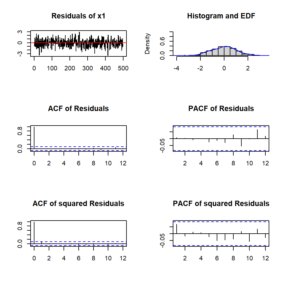.5245

Para \(\hat{a}_1\)

plot(var.serial, names = "x1")

Para \(\hat{a}_2\)

plot(var.serial, names = "x2")

(var.causal.x1<- causality(varsimest,cause="x2"))

$Granger

    Granger causality H0: x2 do not Granger-cause x1

data:  VAR object varsimest
F-Test = 48.707, df1 = 1, df2 = 994, p-value = 5.425e-12


$Instant

    H0: No instantaneous causality between: x2 and x1

data:  VAR object varsimest
Chi-squared = 0.061316, df = 1, p-value = 0.8044

(var.causal.x2<- causality(varsimest,cause="x1"))

$Granger

    Granger causality H0: x1 do not Granger-cause x2

data:  VAR object varsimest
F-Test = 3.6817, df1 = 1, df2 = 994, p-value = 0.0553


$Instant

    H0: No instantaneous causality between: x1 and x2

data:  VAR object varsimest
Chi-squared = 0.061316, df = 1, p-value = 0.8044

Pronóstico

Contenido

VARX(p)
Ejemplo simulado
Pronóstico
El análisis del impulso-respuesta
Ejemplo

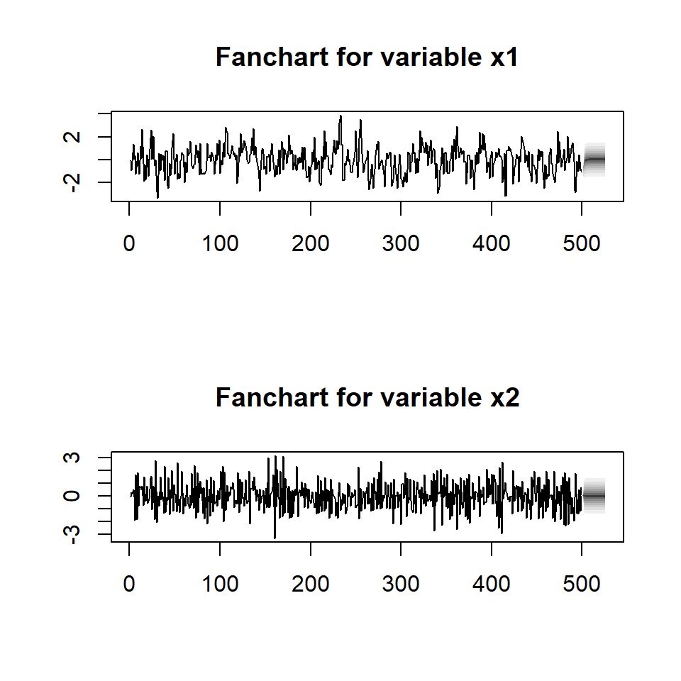
Pronóstico

Dadas las observaciones \(X_1,...,X_T\), el pronóstico \(h\) pasos para frente, \(X_{T+h}\) es dado por

\[X_{T}(h)=CD_{T+h}+\phi_1 X_{T+h-1}+...+\phi_pX_{T+h-p},\] donde \(X_{T}(j)=X_{T+j}\) para \(j\leq 0\).

El error de pronóstico de \(h\) pasos para frente es dado por \[e_h(h)=X_{T+h}-X_{T}(h)\]
El cálculo del error de pronóstico de \(X_{T}(h)\) es más conveniente usar la representación de MA, y el error de pronóstico es dado por

\[X_{T}(h)= a_{T+h} + \phi_1 a_{T+h-1}+...+\phi_{h-1} a_{T+1},\]

Ejemplo

predictions <- predict(varsimest, n.ahead = 25,
                       ci = 0.95)
fanchart(predictions)

El análisis del impulso-respuesta

Contenido

VARX(p)
Ejemplo simulado
Pronóstico
El análisis del impulso-respuesta
Ejemplo

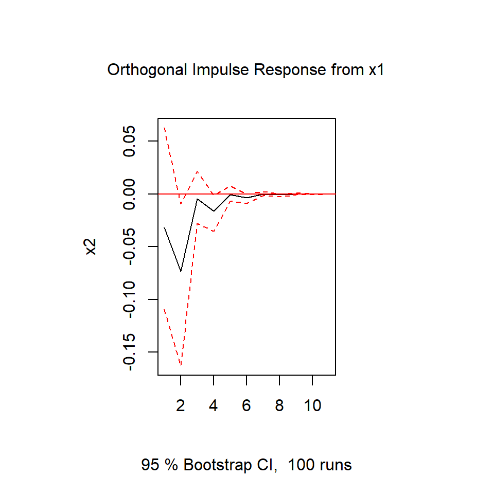
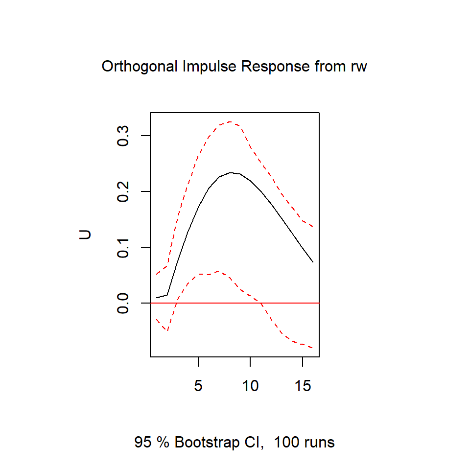
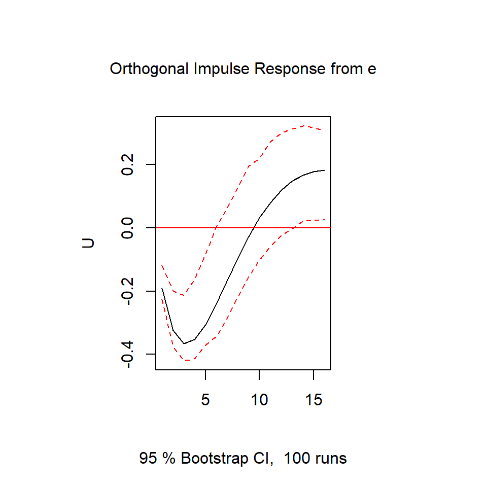
El análisis del impulso-respuesta

Para cualquier modelo VAR(p) estacionario, tiene la representación de MA:

\[X_{t}= \theta_0 a_{t}+\theta_1 a_{t-1}+ \theta_{2} a_{t-2}+...\]

Se interpreta como una regresión en donde cada entrada \((i,j)\) de \(\theta_m,~m=1,...\) representa el cambio del valor esperado de \(X_{j}\) bajo un cambio de una unidad de \(X_i\).
Por ejemplo, para el modelo:

\[\begin{bmatrix}X_{1t}\\ X_{2t} \end{bmatrix} = \begin{bmatrix}\theta_{0,11} & \theta_{0,12} \\ \theta_{0,21} & \theta_{0,22} \end{bmatrix} \begin{bmatrix}a_{1,t}\\ a_{2,t} \end{bmatrix} +\begin{bmatrix}\theta_{1,11} & \theta_{1,12} \\ \theta_{1,21} & \theta_{1,22} \end{bmatrix} \begin{bmatrix}a_{1,t-1}\\ a_{2,t-1} \end{bmatrix}+\dots\]

\(\theta_{1,21}\) representa el cambio del valor esperado de \(X_{2,t+1}\) bajo un cambio de una unidad de \(X_{1,t}\).
\(\theta_{1,12}\) representa el cambio del valor esperado de \(X_{1,t+1}\) bajo un cambio de una unidad de \(X_{2,t}\).

Ejemplo simulado

irf.y1 <- irf(varsimest, impulse = "x1",
              response = "x2", n.ahead = 10,
              cumulative = FALSE)
plot(irf.y1)

irf.y2 <- irf(varsimest, impulse = "x2",
              response = "x1", n.ahead = 10,
              cumulative = FALSE)
plot(irf.y2)

Ejemplo

Contenido

VARX(p)
Ejemplo simulado
Pronóstico
El análisis del impulso-respuesta
Ejemplo

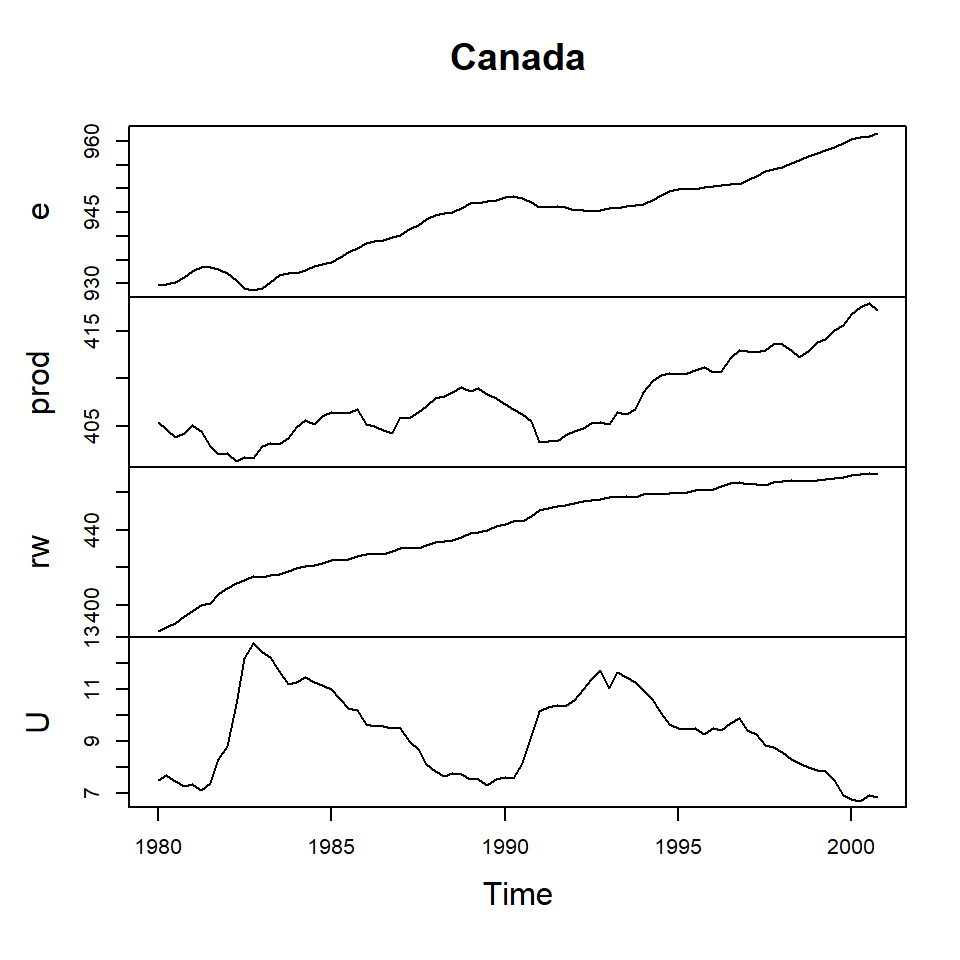
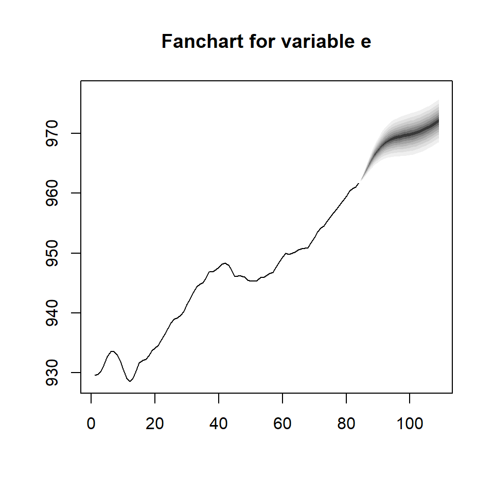
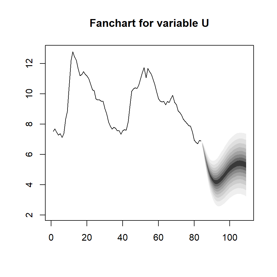
Ejemplo: series macroeconómicas en Canada

Se tienen 4 series de primer trimestre de 1980 al cuarto trimestre de 2000. Se puede interpretar las series como:
- prod: productividad laboral
- e: tasa de empleo
- U: tasa de desempleo
- rw: salario real
Se ajusta un VAR(2) con tendencia.

data(Canada)
plot(Canada)

Estimación

vars::VARselect(Canada, type = "both")

$selection
AIC(n)  HQ(n)  SC(n) FPE(n) 
     3      2      1      3 

$criteria
                  1            2             3            4            5
AIC(n) -6.457999837 -6.862930587 -6.9695915550 -6.826230019 -6.696865092
HQ(n)  -6.159906898 -6.366109023 -6.2740413655 -5.931951204 -5.603857651
SC(n)  -5.710735482 -5.617489996 -5.2259747277 -4.584436956 -3.956895792
FPE(n)  0.001570168  0.001052827  0.0009575467  0.001128994  0.001329669
                  6           7            8            9           10
AIC(n) -6.687175990 -6.55982329 -6.584746129 -6.493397603 -6.523612352
HQ(n)  -5.395439924 -5.06935860 -4.895552811 -4.605475660 -4.436961783
SC(n)  -3.449030454 -2.82350152 -2.350248120 -1.760723357 -1.292761870
FPE(n)  0.001412901  0.00172546  0.001859561  0.002330702  0.002704777

fitvar <- vars::VAR(Canada, p = 2, type = "both")
summary(fitvar)


VAR Estimation Results:
========================= 
Endogenous variables: e, prod, rw, U 
Deterministic variables: both 
Sample size: 82 
Log Likelihood: -170.726 
Roots of the characteristic polynomial:
0.9071 0.9071 0.9037 0.7092 0.7092 0.2549 0.166 0.166
Call:
vars::VAR(y = Canada, p = 2, type = "both")


Estimation results for equation e: 
================================== 
e = e.l1 + prod.l1 + rw.l1 + U.l1 + e.l2 + prod.l2 + rw.l2 + U.l2 + const + trend 

          Estimate Std. Error t value Pr(>|t|)    
e.l1     1.636e+00  1.510e-01  10.830  < 2e-16 ***
prod.l1  1.716e-01  6.280e-02   2.733  0.00789 ** 
rw.l1   -6.006e-02  5.628e-02  -1.067  0.28947    
U.l1     2.740e-01  2.055e-01   1.333  0.18661    
e.l2    -4.842e-01  1.648e-01  -2.938  0.00443 ** 
prod.l2 -9.766e-02  6.747e-02  -1.448  0.15207    
rw.l2    1.689e-03  5.621e-02   0.030  0.97611    
U.l2     1.433e-01  2.108e-01   0.680  0.49886    
const   -1.510e+02  6.921e+01  -2.181  0.03244 *  
trend   -5.706e-03  1.652e-02  -0.345  0.73077    
---
Signif. codes:  0 '***' 0.001 '**' 0.01 '*' 0.05 '.' 0.1 ' ' 1


Residual standard error: 0.365 on 72 degrees of freedom
Multiple R-Squared: 0.9985, Adjusted R-squared: 0.9983 
F-statistic:  5435 on 9 and 72 DF,  p-value: < 2.2e-16 


Estimation results for equation prod: 
===================================== 
prod = e.l1 + prod.l1 + rw.l1 + U.l1 + e.l2 + prod.l2 + rw.l2 + U.l2 + const + trend 

         Estimate Std. Error t value Pr(>|t|)    
e.l1     -0.14817    0.26200  -0.566   0.5735    
prod.l1   1.09881    0.10894  10.087 2.05e-15 ***
rw.l1     0.01519    0.09762   0.156   0.8768    
U.l1     -0.57737    0.35641  -1.620   0.1096    
e.l2      0.23300    0.28585   0.815   0.4177    
prod.l2  -0.21942    0.11703  -1.875   0.0649 .  
rw.l2    -0.09343    0.09750  -0.958   0.3411    
U.l2      0.89061    0.36574   2.435   0.0174 *  
const    -2.16645  120.05179  -0.018   0.9857    
trend     0.06729    0.02865   2.348   0.0216 *  
---
Signif. codes:  0 '***' 0.001 '**' 0.01 '*' 0.05 '.' 0.1 ' ' 1


Residual standard error: 0.6332 on 72 degrees of freedom
Multiple R-Squared: 0.9802, Adjusted R-squared: 0.9777 
F-statistic: 396.4 on 9 and 72 DF,  p-value: < 2.2e-16 


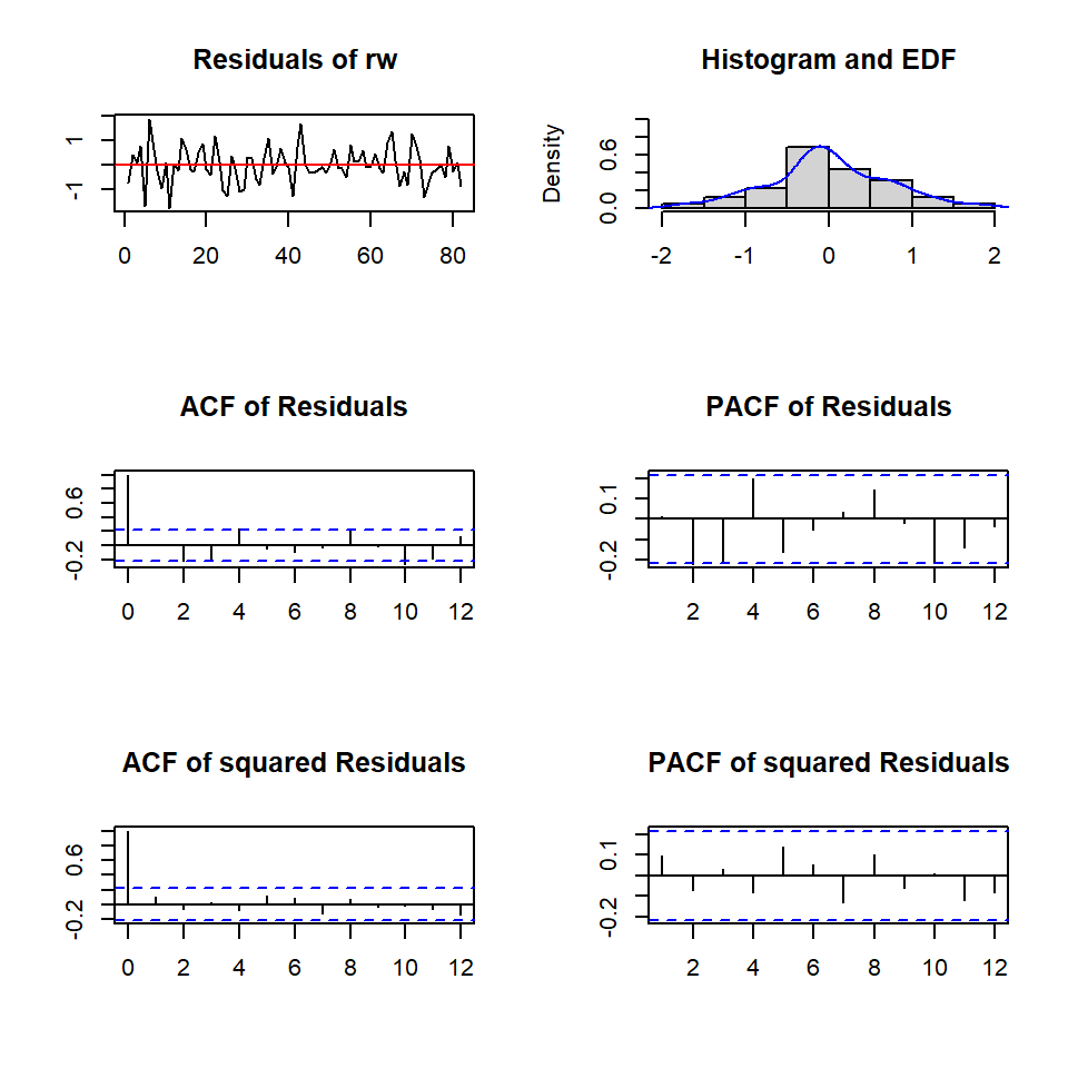
Estimation results for equation rw: 
=================================== 
rw = e.l1 + prod.l1 + rw.l1 + U.l1 + e.l2 + prod.l2 + rw.l2 + U.l2 + const + trend 

         Estimate Std. Error t value Pr(>|t|)    
e.l1     -0.24395    0.31673  -0.770   0.4437    
prod.l1  -0.13328    0.13169  -1.012   0.3149    
rw.l1     0.85895    0.11801   7.279 3.38e-10 ***
U.l1     -0.08787    0.43086  -0.204   0.8390    
e.l2      0.21384    0.34556   0.619   0.5380    
prod.l2  -0.05273    0.14147  -0.373   0.7105    
rw.l2     0.07839    0.11787   0.665   0.5081    
U.l2     -0.25445    0.44213  -0.576   0.5667    
const   133.30872  145.12882   0.919   0.3614    
trend     0.06806    0.03464   1.965   0.0533 .  
---
Signif. codes:  0 '***' 0.001 '**' 0.01 '*' 0.05 '.' 0.1 ' ' 1


Residual standard error: 0.7654 on 72 degrees of freedom
Multiple R-Squared: 0.9989, Adjusted R-squared: 0.9988 
F-statistic:  7398 on 9 and 72 DF,  p-value: < 2.2e-16 


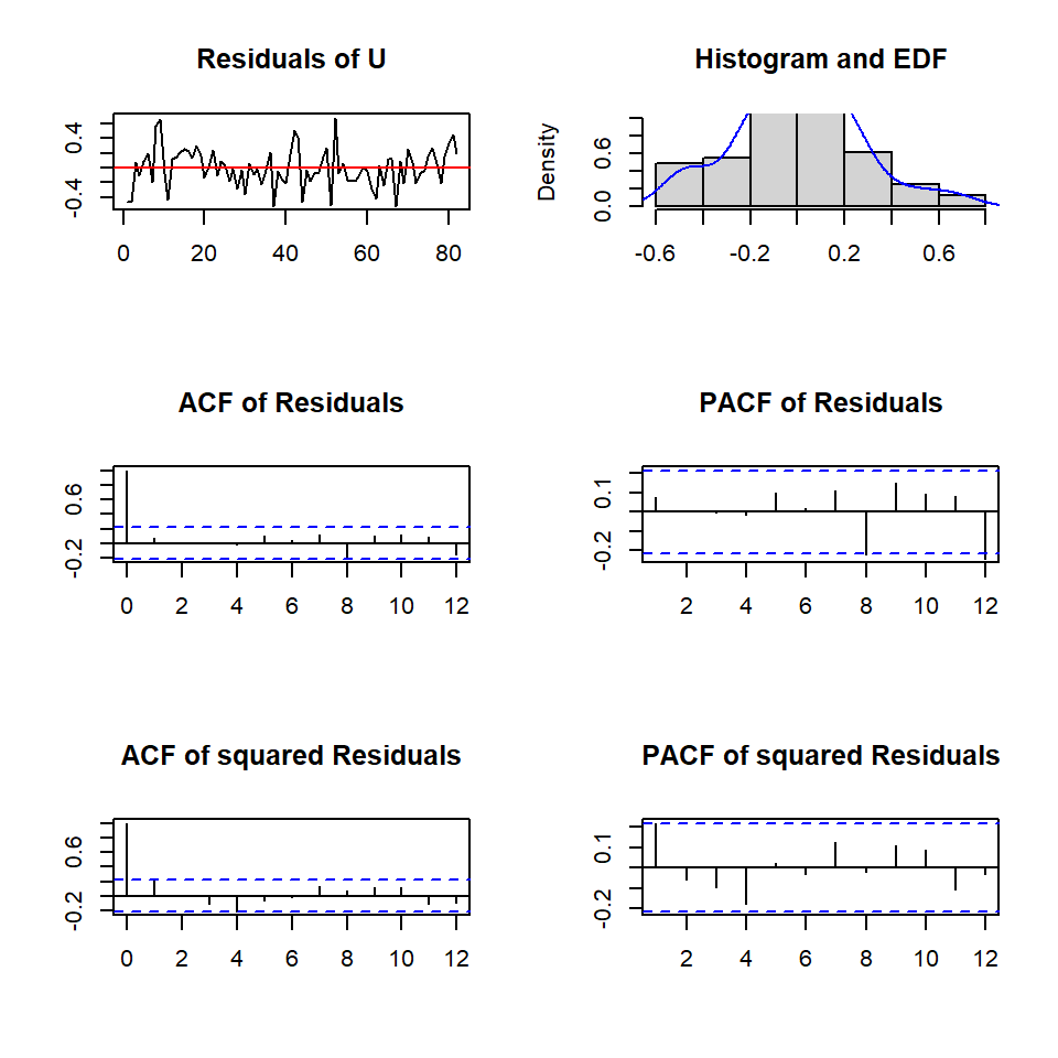
Estimation results for equation U: 
================================== 
U = e.l1 + prod.l1 + rw.l1 + U.l1 + e.l2 + prod.l2 + rw.l2 + U.l2 + const + trend 

         Estimate Std. Error t value Pr(>|t|)    
e.l1     -0.57610    0.11571  -4.979 4.23e-06 ***
prod.l1  -0.08790    0.04811  -1.827 0.071824 .  
rw.l1     0.01182    0.04311   0.274 0.784807    
U.l1      0.60019    0.15740   3.813 0.000287 ***
e.l2      0.38095    0.12624   3.018 0.003520 ** 
prod.l2   0.04321    0.05168   0.836 0.405937    
rw.l2     0.04662    0.04306   1.083 0.282552    
U.l2     -0.09492    0.16152  -0.588 0.558584    
const   180.98536   53.01834   3.414 0.001056 ** 
trend     0.01276    0.01265   1.008 0.316798    
---
Signif. codes:  0 '***' 0.001 '**' 0.01 '*' 0.05 '.' 0.1 ' ' 1


Residual standard error: 0.2796 on 72 degrees of freedom
Multiple R-Squared: 0.973,  Adjusted R-squared: 0.9696 
F-statistic: 288.2 on 9 and 72 DF,  p-value: < 2.2e-16 



Covariance matrix of residuals:
             e      prod       rw         U
e     0.133242 -0.004968 -0.04005 -0.069553
prod -0.004968  0.400914  0.03445  0.008295
rw   -0.040049  0.034449  0.58590  0.028808
U    -0.069553  0.008295  0.02881  0.078193

Correlation matrix of residuals:
           e     prod       rw        U
e     1.0000 -0.02150 -0.14334 -0.68142
prod -0.0215  1.00000  0.07108  0.04685
rw   -0.1433  0.07108  1.00000  0.13459
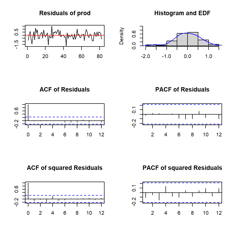
U    -0.6814  0.04685  0.13459  1.00000

Los diagnósticos

(var.serial <- serial.test(fitvar, lags.pt = 16, type = "PT.asymptotic"))


    Portmanteau Test (asymptotic)

data:  Residuals of VAR object fitvar
Chi-squared = 209.74, df = 224, p-value = 0.7443

(var.arch <- arch.test(fitvar, lags.multi = 5, multivariate.only = TRUE))


    ARCH (multivariate)

data:  Residuals of VAR object fitvar
Chi-squared = 528.14, df = 500, p-value = 0.1855

(var.norm <- normality.test(fitvar, multivariate.only = TRUE))

$JB

    JB-Test (multivariate)

data:  Residuals of VAR object fitvar
Chi-squared = 2.465, df = 8, p-value = 0.9633


$Skewness

    Skewness only (multivariate)

data:  Residuals of VAR object fitvar
Chi-squared = 1.3722, df = 4, p-value = 0.849


$Kurtosis

    Kurtosis only (multivariate)

data:  Residuals of VAR object fitvar
Chi-squared = 1.0928, df = 4, p-value = 0.8954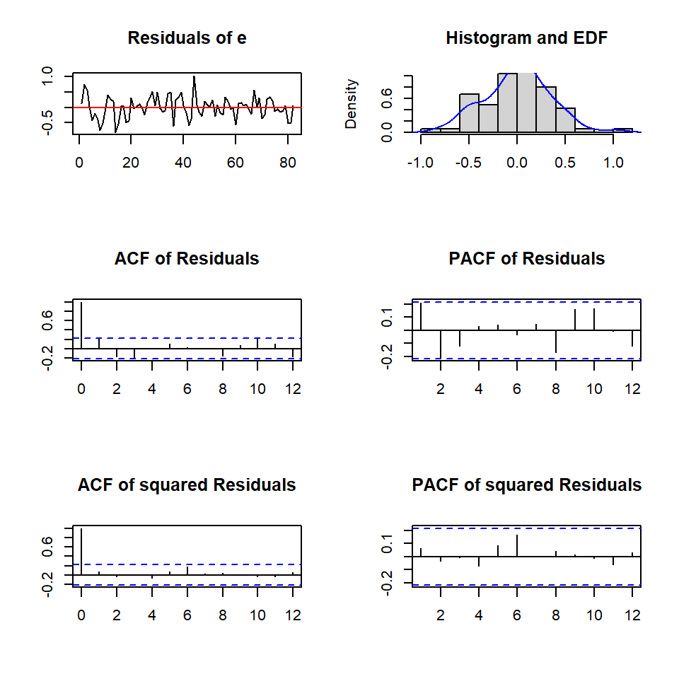

Para \(\hat{a}_1\)

plot(var.serial, names = "e")

Para \(\hat{a}_2\)

plot(var.serial, names = "prod")

Para \(\hat{a}_1\)

plot(var.serial, names = "rw")

Para \(\hat{a}_2\)

plot(var.serial, names = "U")

Causalidad de Granger

(var.causal.1<- causality(fitvar,cause=c("prod", "e", "rw")))

$Granger

    Granger causality H0: e prod rw do not Granger-cause U

data:  VAR object fitvar
F-Test = 8.5625, df1 = 6, df2 = 288, p-value = 1.422e-08


$Instant

    H0: No instantaneous causality between: e prod rw and U

data:  VAR object fitvar
Chi-squared = 26.088, df = 3, p-value = 9.139e-06

(var.causal.2<- causality(fitvar,cause=c("prod","rw")))

$Granger

    Granger causality H0: prod rw do not Granger-cause e U

data:  VAR object fitvar
F-Test = 2.964, df1 = 8, df2 = 288, p-value = 0.003337


$Instant

    H0: No instantaneous causality between: prod rw and e U

data:  VAR object fitvar
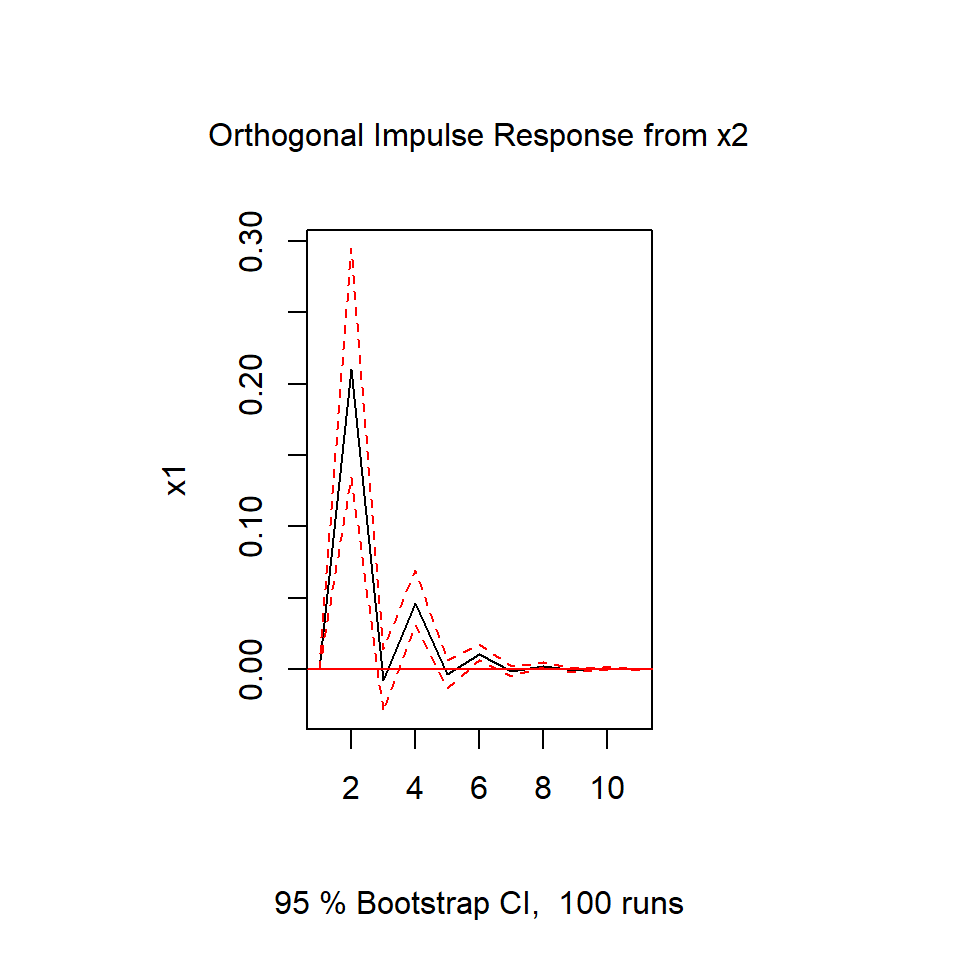
Chi-squared = 1.9934, df = 4, p-value = 0.737

Análisis del impulso-respuesta

irf1 <- irf(fitvar, impulse = "rw",
              response = "U", n.ahead = 15,
              cumulative = FALSE)
plot(irf1)

irf2 <- irf(fitvar, impulse = "e",
              response = "U", n.ahead = 15,
              cumulative = FALSE)
plot(irf2)

Predicciones

predictions <- predict(fitvar, n.ahead = 25,
                       ci = 0.95)
fanchart(predictions, name= "e")

fanchart(predictions, name= "U")

Paquetes en R

Para replicar los ejemplos de esta presentación, necesitan estos paquetes:

library(ggplot2)
library(tidyverse)
library(vars)
library(MASS)
library(MTS)

Tema 2: Análisis multivariado de series temporales(3)

VARX(p)

VARX(p)

VARX(1)

Causalidad de Granger de un VAR(1)

Causalidad de Granger de un VARX(p)

Causalidad de Granger de VAR(1) con \(k=3\)

Ejemplo simulado

Ejemplo simulado

Estimación de modelos

Los diagnósticos

Pronóstico

Pronóstico

Ejemplo

El análisis del impulso-respuesta

El análisis del impulso-respuesta

Ejemplo simulado

Ejemplo

Ejemplo: series macroeconómicas en Canada

Estimación

Los diagnósticos

Causalidad de Granger

Análisis del impulso-respuesta

Predicciones

Paquetes en R

Tema 2: Análisis multivariado de series temporales⁽³⁾