lab05a: Bootstrap

XS3310 Teoría Estadística

Autor/a

Afiliación

Shu Wei Chou Chen

Escuela de Estadística (UCR)

Este documento ilustra el uso de Bootstrap.

Se tienen datos de sobrevivencia de 16 ratones luego de una cirugía de prueba: 9 ratones en el grupo control y 7 ratones en el grupo de tratamiento.

Grupo	Tiempo de sovrevivencia(días)	Media
Tratamiento	94,197,16,38,99,141,23	86.86
Control	52,104,146,10,51,30,40,27,46	56.22

¿Podemos decir que el tratamiento es efectivo?

En estadística, resolvemos esa pregunta estimando \(\bar{X}- \bar{Y} = 30.63\). El problema es cómo calcular la variabilidad, ¿podemos suponer lo mismo de siempre?

1 Datos

X<-c(94,197,16,38,99,141,23)
Y<-c(52,104,146,10,51,30,40,27,46)

2 Estimación de \(\bar{X}\).

2.1 Estimación por intervalo del tiempo promedio de sobrevivencia del tratamiento.

(estimacion<-mean(X))

[1] 86.85714

sd(X)

[1] 66.76683

n<-length(X)

Asumiendo normalidad de la población, tenemos que el intervalo de confianza de 95% es dado por:

estimacion+c(-1,1)*qt(p=0.975,df=(n-1))*sd(X)/sqrt(n)

[1]  25.10812 148.60616

2.2 IC estándar de Bootstrap

B <- 1000
Tboot_b <- NULL
for(b in 1:B) {
  xb <- sample(X, size = n, replace = TRUE)
  Tboot_b[b] <- mean(xb)
}
Tboot_b[1:10]

 [1]  84.00000  86.57143  99.57143  91.28571  90.00000  83.00000 105.42857
 [8]  88.14286 115.57143  72.14286

hist(Tboot_b)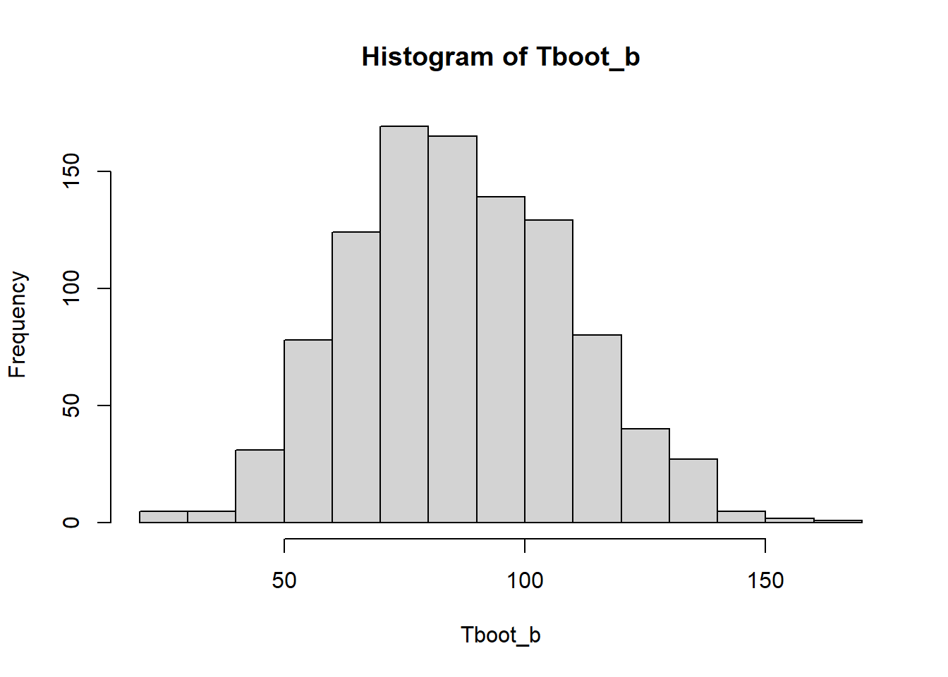

2.2.1 Sesgo del bootstrap

(media_bootstrap <- mean(Tboot_b))

[1] 86.69243

estimacion

[1] 86.85714

(sesgo_bootstrap <- media_bootstrap-estimacion)

[1] -0.1647143

2.2.2 Intervalos de confianza de 95%

(cuantil_z <- qnorm(1 - 0.05 / 2))

[1] 1.959964

(sdboot <- sd(Tboot_b))

[1] 22.59721

estimacion + c(-1,1)*cuantil_z * sdboot

[1]  42.56742 131.14687

2.2.3 IC bootstrap t

B <- 1000
Tboot_b <- NULL
Tboot_bm <- NULL
sdboot_b <- NULL
for (b in 1:B) {
  xb <- sample(X, size = n, replace = TRUE)
  Tboot_b[b] <- mean(xb)
  for (m in 1:B) {
    xbm <- sample(xb, size = n, replace = TRUE)
    Tboot_bm[m] <- mean(xbm)
  }
  sdboot_b[b] <- sd(Tboot_bm)
}
z_star <- (Tboot_b - estimacion) / sdboot_b

hist(z_star)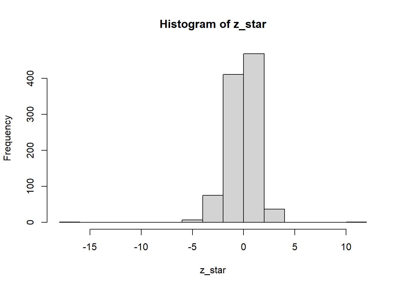

summary(z_star)

     Min.   1st Qu.    Median      Mean   3rd Qu.      Max. 
-16.08554  -0.82876   0.02683  -0.10469   0.76720  10.80232

cuantil_t_empirico <- quantile(z_star, c(0.05/2, 1-0.05/2))
estimacion +cuantil_t_empirico* sdboot

     2.5%     97.5% 
 10.24223 134.78094

2.2.4 IC percentil de bootstrap

B <- 1000
Tboot_b <- NULL
for(b in 1:B) {
  xb <- sample(X, size = n, replace = TRUE)
  Tboot_b[b] <- mean(xb)
}
hist(Tboot_b)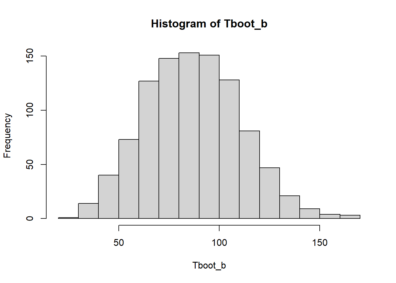

quantile(Tboot_b,0.05 / 2)

    2.5% 
43.84643

quantile(Tboot_b, 1 - 0.05 / 2)

   97.5% 
134.4714

2.2.5 Con el paquete `boots` de R.

library(boot)

Warning: package 'boot' was built under R version 4.3.3

mean_fun=function(datos,indice){ 
  m=mean(datos[indice]) 
  v=var(datos[indice]) 
  c(m,v)
}

X.boot<-boot(X,mean_fun,R=1000) 
(results<-boot.ci(X.boot,type=c("basic","stud","perc")))

BOOTSTRAP CONFIDENCE INTERVAL CALCULATIONS
Based on 1000 bootstrap replicates

CALL : 
boot.ci(boot.out = X.boot, type = c("basic", "stud", "perc"))

Intervals : 
Level      Basic             Studentized          Percentile     
95%   ( 39.59, 130.29 )   ( 31.93, 165.10 )   ( 43.43, 134.12 )  
Calculations and Intervals on Original Scale

3 Estimación de \(\bar{X}\) - \(\bar{Y}\).

3.1 Ilustración a mano

(estimacion<-mean(X)-mean(Y))

[1] 30.63492

n<-length(X)
m<-length(Y)
B <- 1000
Tboot_b <- NULL
for(b in 1:B) {
  xb <- sample(X, size = n, replace = TRUE)
  yb <- sample(Y, size = m, replace = TRUE)
  Tboot_b[b] <- mean(xb)-mean(yb)
}
Tboot_b[1:10]

 [1] 32.1269841 35.4920635 42.6190476 33.0952381 32.0158730  6.5555556
 [7] 33.4920635  0.6031746  4.0793651 10.5714286

hist(Tboot_b)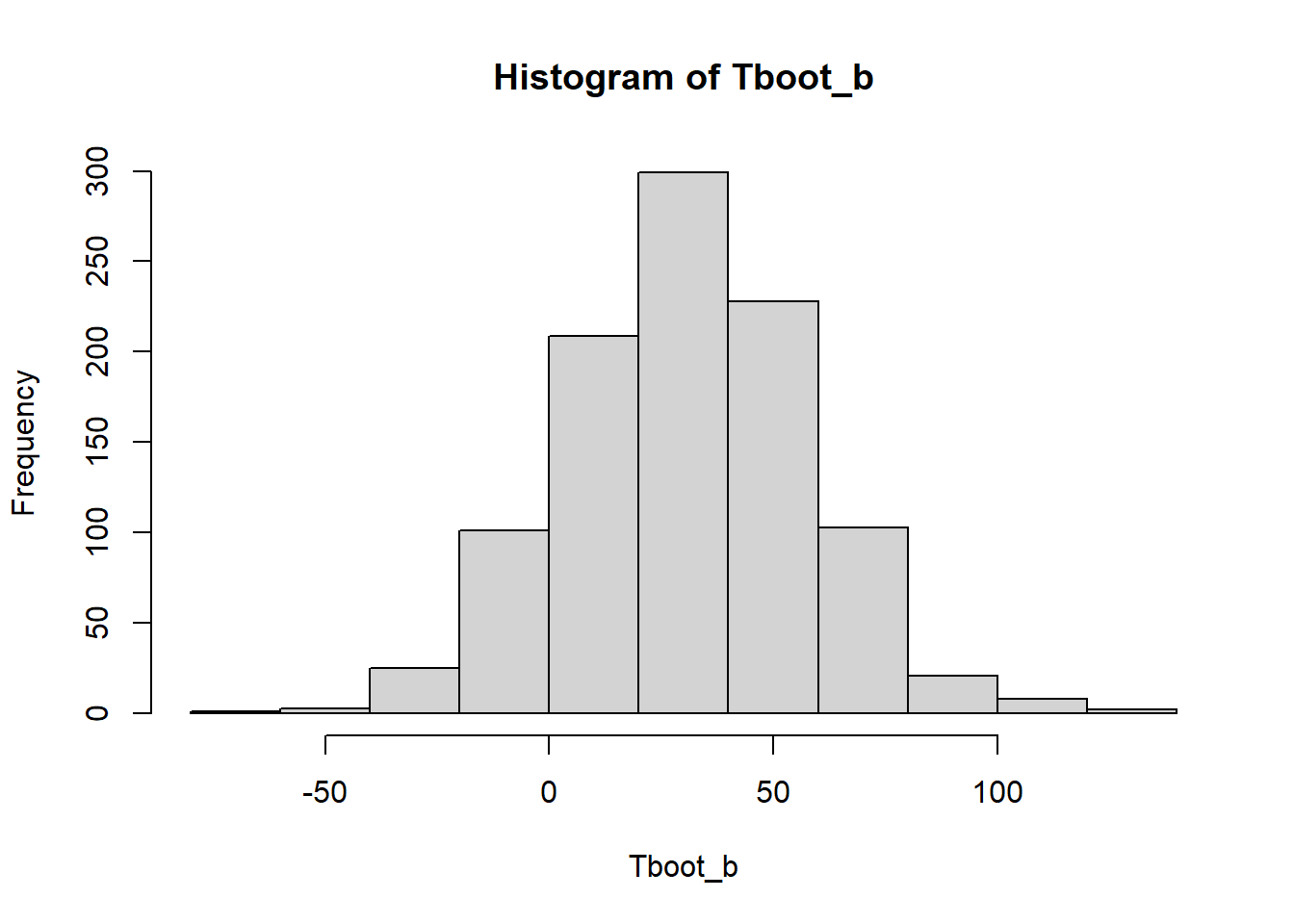

(cuantil_z <- qnorm(1 - 0.05 / 2))

[1] 1.959964

(sdboot <- sd(Tboot_b))

[1] 27.28183

estimacion + c(-1,1)*cuantil_z * sdboot

[1] -22.83648  84.10632

3.2 Con el paquete `simpleboot`

library(simpleboot)

Warning: package 'simpleboot' was built under R version 4.3.3

Simple Bootstrap Routines (1.1-7)

bootstrap_diff <- two.boot(X, Y, mean, R = 1000, student = TRUE, M = 1000)
(bootstrap_diff_res<-boot.ci(bootstrap_diff,type=c("basic","stud","perc")))

BOOTSTRAP CONFIDENCE INTERVAL CALCULATIONS
Based on 1000 bootstrap replicates

CALL : 
boot.ci(boot.out = bootstrap_diff, type = c("basic", "stud", 
    "perc"))

Intervals : 
Level      Basic             Studentized          Percentile     
95%   (-23.24,  80.38 )   (-29.88, 102.24 )   (-19.11,  84.51 )  
Calculations and Intervals on Original Scale