Fitting Additive partial linear models with symmetric errors

aplms fits additive partial linear models with autoregressive symmetric errors. This method is suitable for data sets where the response variable is continuous and symmetric, with either heavy or light tails, and measured over time. The model includes a parametric component for a set of covariates, while another set of covariates can be specified as semi-parametric functions, typically time-related. In this setup, natural cubic splines or cubic P-splines are used to approximate the nonparametric components.

Usage

aplms(
  formula,
  npc,
  basis,
  Knot,
  data,
  family = Normal(),
  p = 1,
  control = list(tol = 0.001, algorithm1 = c("P-GAM"), algorithm2 = c("BFGS"), Maxiter1 =
    20, Maxiter2 = 25),
  init,
  lam,
  verbose = FALSE
)

# S3 method for class 'aplms'
print(x, ...)

Arguments

formula: A symbolic description of the parametric component of the model to be fitted. The details of model specification are given under ‘Details’.
npc: A vector of names of non parametric component.
basis: A vector of names of the basis to be used for each non parametric covariate.
Knot: A vector of the number of knots in each non-linear component of the model.
data: A data frame containing the variables in the model
family: Symmetric error distribution. The implemented distribution are: Normal(), LogisI(), LogisII(), Student(df), Powerexp(k), Gstudent(parm=c(s,r)).
p: autoregressive order of the error
control: optimization rutine.
init: A list of initial values for the symmetric error scale, phi, and autoregressive coefficients, rhos.
lam: smoothing parameter vector.
verbose: Logical; if TRUE, prints estimation progress messages. Default is FALSE.
x: APLMS object.
...: other arguments

Value

Returns an object of class “aplms”, a list with following components.

formula: the formula object used.
family: the family object used.
npc: the npc object used.
Knot: the Knot object used.
lam: the lam object used.
rdf: Degrees of freedom: n - q - p - 1.
VAR_F: Estimate the asymptotic covariance matrix for the gamma parameters.
basis: The basis to be used for each non parametric covariate.
WALD_f: The summary table of the Wald statistics.
summary_table_phirho: The summary table of the rho and phi parameters.
N_i: Basis functions.
f: Estimated gamma parameters.
Dv: Dv values for the symmetric error.
Dm: Dm values for the symmetric error.
Dc: Dc values for the symmetric error.
Dd: Dd values for the symmetric error.
delta: delta_i for the symmetric error.
LL_obs: Observed information matrix of the fitted model.
loglike: The estimated loglikelihood function of the fitted model.
total_df: The total effective degree of freedom of the model.
parametric_df: The degree of freedom of the parametric components.
npc_df: The effective degree of freedom of the non parametric components.
AIC: Akaike information criterion of the estimated model.
BIC: Bayesian information criterion of the estimated model.
AICC: Corrected Akaike information criterion of the estimated model.
GCV: The generalized cross-validation (GCV).
yhat: The fitted response values of the model.
muhat: The fitted mean values of the model.
residuals_y: The response residuals
residuals_mu: Raw (Ordinary) residuals: \(y_t - (\textbf{x}_i^\top\beta + f_1(t_{i1}) + \ldots + f_k(t_{ik}))\)
data: the data object used.
this.call: the function call used.

References

Chou-Chen, S.W., Oliveira, R.A., Raicher, I., Gilberto A. Paula (2024) Additive partial linear models with autoregressive symmetric errors and its application to the hospitalizations for respiratory diseases Stat Papers 65, 5145–5166. doi:10.1007/s00362-024-01590-w

Oliveira, R.A., Paula, G.A. (2021) Additive partial linear models with autoregressive symmetric errors and its application to the hospitalizations for respiratory diseases Comput Stat 36, 2435–2466. doi:10.1007/s00180-021-01106-2

Examples

data(temperature)
temperature.df = data.frame(temperature,time=1:length(temperature))
model<-aplms::aplms(temperature ~ 1,
                   npc=c("time"), basis=c("cr"),Knot=c(60),
                   data=temperature.df,family=Powerexp(k=0.3),p=1,
                   control = list(tol = 0.001,
                                  algorithm1 = c("P-GAM"),
                                  algorithm2 = c("BFGS"),
                                  Maxiter1 = 20,
                                  Maxiter2 = 25),
                   lam=c(10))
plot(model)

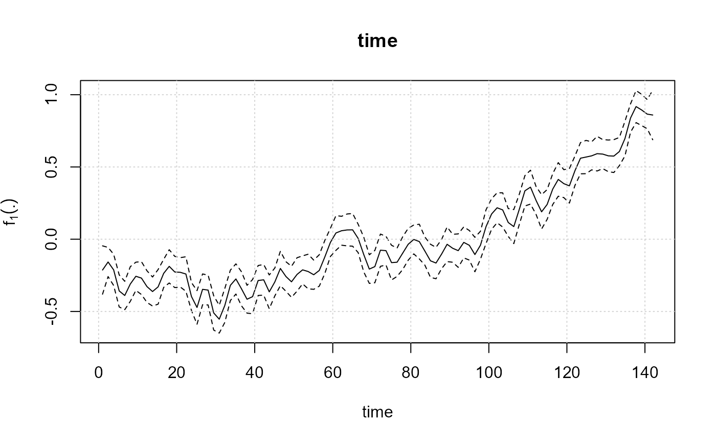#> [[1]]
#>            cov        fmean    fmean_ls     fmean_li
#> 1     1.000000 -0.213215062 -0.38051702 -0.045913101
#> 2     2.424242 -0.157657300 -0.25860288 -0.056711725
#> 3     3.848485 -0.212090507 -0.32001771 -0.104163305
#> 4     5.272727 -0.357959506 -0.46898184 -0.246937174
#> 5     6.696970 -0.389381087 -0.48749987 -0.291262301
#> 6     8.121212 -0.309883662 -0.42979400 -0.189973326
#> 7     9.545455 -0.256507180 -0.35408994 -0.158924423
#> 8    10.969697 -0.268972025 -0.38269634 -0.155247707
#> 9    12.393939 -0.328028685 -0.43751976 -0.218537614
#> 10   13.818182 -0.362119686 -0.46252234 -0.261717030
#> 11   15.242424 -0.329739301 -0.44963766 -0.209840943
#> 12   16.666667 -0.236456854 -0.33345593 -0.139457776
#> 13   18.090909 -0.187783201 -0.30292439 -0.072642015
#> 14   19.515152 -0.226748006 -0.33476704 -0.118728976
#> 15   20.939394 -0.229175092 -0.33080619 -0.127543993
#> 16   22.363636 -0.240824195 -0.36025925 -0.121389135
#> 17   23.787879 -0.396329451 -0.49288877 -0.299770132
#> 18   25.212121 -0.472299770 -0.58853860 -0.356060937
#> 19   26.636364 -0.346859356 -0.45344989 -0.240268819
#> 20   28.060606 -0.352051750 -0.45504127 -0.249062233
#> 21   29.484848 -0.509917727 -0.62863393 -0.391201528
#> 22   30.909091 -0.553447782 -0.64976105 -0.457134516
#> 23   32.333333 -0.458669461 -0.57595336 -0.341385561
#> 24   33.757576 -0.319163400 -0.42430868 -0.214018119
#> 25   35.181818 -0.274962044 -0.37937956 -0.170544531
#> 26   36.606061 -0.343014587 -0.46081001 -0.225219168
#> 27   38.030303 -0.415401411 -0.51166773 -0.319135092
#> 28   39.454545 -0.397422379 -0.51569997 -0.279144793
#> 29   40.878788 -0.285716394 -0.38941287 -0.182019919
#> 30   42.303030 -0.281039407 -0.38691070 -0.175168109
#> 31   43.727273 -0.364210514 -0.48097224 -0.247448788
#> 32   45.151515 -0.295850803 -0.39226072 -0.199440886
#> 33   46.575758 -0.202393200 -0.32149651 -0.083289890
#> 34   48.000000 -0.258064413 -0.36036400 -0.155764823
#> 35   49.424242 -0.294762948 -0.40206745 -0.187458442
#> 36   50.848485 -0.243743271 -0.35944671 -0.128039829
#> 37   52.272727 -0.212056003 -0.30881412 -0.115297886
#> 38   53.696970 -0.223624912 -0.34332922 -0.103920599
#> 39   55.121212 -0.245821845 -0.34682625 -0.144817439
#> 40   56.545455 -0.216226869 -0.32497022 -0.107483516
#> 41   57.969697 -0.122563126 -0.23710176 -0.008024492
#> 42   59.393939 -0.022064966 -0.11936732  0.075237389
#> 43   60.818182  0.043246936 -0.07680916  0.163303035
#> 44   62.242424  0.058536017 -0.04133763  0.158409663
#> 45   63.666667  0.064177908 -0.04607577  0.174431583
#> 46   65.090909  0.064875182 -0.04834389  0.178094259
#> 47   66.515152  0.005296521 -0.09272732  0.103320363
#> 48   67.939394 -0.105963819 -0.22614647  0.014218833
#> 49   69.363636 -0.206727445 -0.30561597 -0.107838917
#> 50   70.787879 -0.189575482 -0.30134938 -0.077801580
#> 51   72.212121 -0.076046167 -0.18782007  0.035727734
#> 52   73.636364 -0.079103697 -0.17799222  0.019784831
#> 53   75.060606 -0.162040947 -0.28222360 -0.041858296
#> 54   76.484848 -0.159214768 -0.25723861 -0.061190926
#> 55   77.909091 -0.096978598 -0.21019767  0.016240479
#> 56   79.333333 -0.034892264 -0.14514594  0.075361411
#> 57   80.757576 -0.001654978 -0.10152862  0.098218668
#> 58   82.181818 -0.016382605 -0.13643870  0.103673494
#> 59   83.606061 -0.082110591 -0.17941295  0.015191763
#> 60   85.030303 -0.149307173 -0.26384581 -0.034768540
#> 61   86.454545 -0.164889347 -0.27363270 -0.056145994
#> 62   87.878788 -0.103394785 -0.20439919 -0.002390379
#> 63   89.303030 -0.035126676 -0.15483099  0.084577636
#> 64   90.727273 -0.062581265 -0.15933938  0.034176852
#> 65   92.151515 -0.079086931 -0.19479037  0.036616512
#> 66   93.575758 -0.021958536 -0.12926304  0.085345970
#> 67   95.000000 -0.042156899 -0.14445649  0.060142691
#> 68   96.424242 -0.106105596 -0.22520891  0.012997714
#> 69   97.848485 -0.041483460 -0.13789338  0.054926457
#> 70   99.272727  0.086897127 -0.02986460  0.203658853
#> 71  100.696970  0.174316765  0.06844547  0.280188063
#> 72  102.121212  0.217565731  0.11386926  0.321262206
#> 73  103.545455  0.202671643  0.08439406  0.320949227
#> 74  104.969697  0.115659933  0.01939361  0.211926256
#> 75  106.393939  0.087320078 -0.03047534  0.205115498
#> 76  107.818182  0.208210642  0.10379313  0.312628152
#> 77  109.242424  0.335094675  0.22994939  0.440239956
#> 78  110.666667  0.360344269  0.24306036  0.477628175
#> 79  112.090909  0.268794480  0.17248123  0.365107728
#> 80  113.515152  0.189627094  0.07091091  0.308343273
#> 81  114.939394  0.240639673  0.13765014  0.343629210
#> 82  116.363636  0.346623508  0.24003297  0.453214045
#> 83  117.787879  0.413779514  0.29754069  0.530018341
#> 84  119.212121  0.384577682  0.28801824  0.481137123
#> 85  120.636364  0.369334466  0.24989923  0.488769704
#> 86  122.060606  0.473909701  0.37227863  0.575540771
#> 87  123.484848  0.560667717  0.45264868  0.668686751
#> 88  124.909091  0.568661309  0.45351981  0.683802810
#> 89  126.333333  0.576904017  0.47990550  0.673902532
#> 90  127.757576  0.592069051  0.47217142  0.711966684
#> 91  129.181818  0.589034350  0.48862971  0.689438988
#> 92  130.606061  0.577041729  0.46755078  0.686532679
#> 93  132.030303  0.575296888  0.46156731  0.689026471
#> 94  133.454545  0.606978315  0.50938891  0.704567721
#> 95  134.878788  0.696587825  0.57665900  0.816516648
#> 96  136.303030  0.838493153  0.74033856  0.936647746
#> 97  137.727273  0.917933747  0.80690816  1.028959338
#> 98  139.151515  0.894514412  0.78638554  1.002643279
#> 99  140.575758  0.865726591  0.76474733  0.966705850
#> 100 142.000000  0.859592517  0.68831338  1.030871657
#> 
summary(model)
#>  ---------------------------------------------------------------
#>  Additive partial linear models with symmetric errors 
#>  ---------------------------------------------------------------
#>  Sample size:  142 
#>  -------------------------- Model ---------------------------
#> 
#> aplms::aplms(formula = temperature ~ 1, npc = c("time"), basis = c("cr"), 
#>     Knot = c(60), data = temperature.df, family = Powerexp(k = 0.3), 
#>     p = 1, control = list(tol = 0.001, algorithm1 = c("P-GAM"), 
#>         algorithm2 = c("BFGS"), Maxiter1 = 20, Maxiter2 = 25), 
#>     lam = c(10))
#>  
#>  ------------------- Parametric component -------------------
#> 
#>           Estimate Std. Error t value  Pr(>|t|)    
#> intercept 0.056619     0.0041 13.8905 < 2.2e-16 ***
#> 
#>  ----------------- Non-parametric component ------------------ 
#> 
#>          Wald       df    Pr(>.)    
#> time 7589.838   58.583 < 2.2e-16 ***
#> 
#>  --------------- Autoregressive and Scale parameter ---------------- 
#> 
#>        Estimate Std. Error    Wald  Pr(>|t|)    
#> phi   0.0022992     0.0003  7.3902 1.242e-11 ***
#> rho1 -0.2571215     0.0662 -3.8866 0.0001568 ***
#>  
#> 
#> ------ Penalized Log-likelihood and Information criterion------
#> 
#>  Log-lik:  200.07 
#>  AIC    :  -276.97 
#>  AICc   :  -274.46 
#>  BIC    :  -94.94 
#>  GCV    :  0.01 
#> 
#>  --------------------------------------------------------------------
print(model)
#> Call:
#> aplms::aplms(formula = temperature ~ 1, npc = c("time"), basis = c("cr"), 
#>     Knot = c(60), data = temperature.df, family = Powerexp(k = 0.3), 
#>     p = 1, control = list(tol = 0.001, algorithm1 = c("P-GAM"), 
#>         algorithm2 = c("BFGS"), Maxiter1 = 20, Maxiter2 = 25), 
#>     lam = c(10))