Diagnostic Plots for additive partial linear models with symmetric errors

Usage

aplms.diag.plot(model, which, labels = NULL, iden = FALSE, ...)

Arguments

model: an object with the result of fitting additive partial linear models with symmetric errors.
which: an optional numeric value with the number of only plot that must be returned.
labels: a optional string vector specifying a labels plots.
iden: a logical value used to identify observations. If TRUE the observations are identified by user in the graphic window.
...: graphics parameters to be passed to the plotting routines.

Value

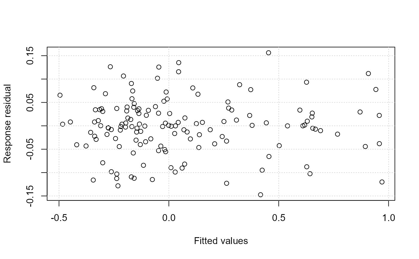
Return an interactive menu with eleven options to make plots. This menu contains the follows graphics: 1: Response residuals against fited values. 2: Response residuals against time index. 3: Histogram of Response residuals. 4: Autocorrelation function of response residuals. 5: Partial autocorrelation function of response residuals. 6: Conditional quantile residuals against fited values. 7: Conditional quantile residuals against time index. 8: Histogram of conditional quantile residuals. 9: Autocorrelation function of conditional quantile residual. 10: Partial autocorrelation function of conditional quantile residuals. 11: QQ-plot of conditional quantile residuals.

Examples

data(temperature)
temperature.df = data.frame(temperature,time=1:length(temperature))
model<-aplms::aplms(temperature ~ 1,
                   npc=c("time"), basis=c("cr"),Knot=c(60),
                   data=temperature.df,family=Powerexp(k=0.3),p=1,
                   control = list(tol = 0.001,
                                  algorithm1 = c("P-GAM"),
                                  algorithm2 = c("BFGS"),
                                  Maxiter1 = 20,
                                  Maxiter2 = 25),
                   lam=c(10))
aplms.diag.plot(model, which = 1)
#> Registered S3 method overwritten by 'rmutil':
#>   method         from 
#>   plot.residuals psych