Local influence plots of the object `aplms()` — influenceplot.aplms • aplms

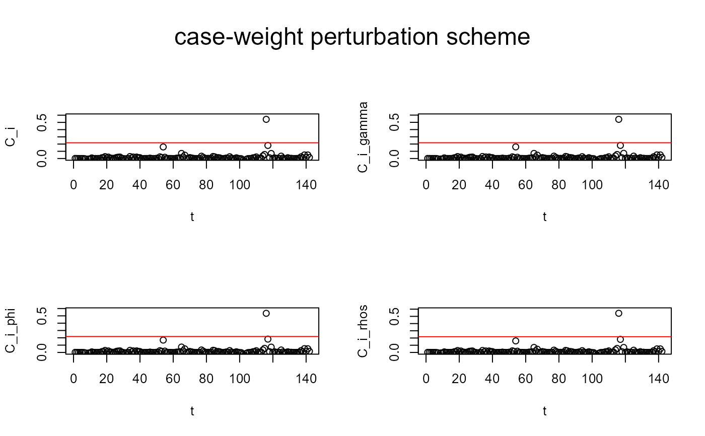
Takes a fitted `aplms` object and outputs diagnostics of the sensitivity analysis by assessing the effects of perturbations in the model and/or data, on the parameter estimates. The `case-weight`, `dispersion`, `response`, `explanatory`, and `corAR` perturbations are available.

Usage

influenceplot.aplms(
  model,
  perturbation = c("case-weight", "dispersion", "response", "explanatory", "corAR"),
  part = TRUE,
  C = 4,
  labels = NULL
)

Arguments

model: an object with the result of fitting additive partial linear models with symmetric errors.
perturbation: A string vector specifying a perturbation scheme: `case-weight`, `dispersion`, `response`, `explanatory`, and `corAR`.
part: A logical value to indicate whether the influential analysis is performed for \(\gamma\), \(\phi\) and \(\rho\).
C: The cutoff criterion such that \(C_i > \bar{C_i} + C*sd(C_i)\) to detect influential observations.
labels: label to especify each data point.

Value

The conformal normal curvature of the specified perturbations is plotted.

Examples

data(temperature)
temperature.df = data.frame(temperature,time=1:length(temperature))
model<-aplms::aplms(temperature ~ 1,
                   npc=c("time"), basis=c("cr"),Knot=c(60),
                   data=temperature.df,family=Powerexp(k=0.3),p=1,
                   control = list(tol = 0.001,
                                  algorithm1 = c("P-GAM"),
                                  algorithm2 = c("BFGS"),
                                  Maxiter1 = 20,
                                  Maxiter2 = 25),
                   lam=c(10))
influenceplot.aplms(model, perturbation = c("case-weight"))
#> [1] "case-weight perturbation scheme"